This story was published by Towards AI.
Imagine trying to find a needle in a digital haystack of millions of data points. In the world of AI and machine learning, choosing the right vector index is akin to equipping yourself with a magnet — it can make the search not only faster but also more accurate. Whether you’re building a recommendation system, a chatbot, or any Retrieval-Augmented Generation (RAG) application, the vector index you choose can significantly impact performance. So, how do you make the right choice? Let’s dive in.
What is Similarity Search?
Before we delve into vector indexes, it’s essential to understand similarity search. Similarity search aims to find items that are similar to a given query item, based on some defined criteria or distance metric. In machine learning, this often involves comparing high-dimensional vectors that represent data points like images, text embeddings, or user preferences.
What is a Vector Index?
Think of a vector index as a specialized filing system for high-dimensional data. Just like a library index helps you find a book quickly among thousands, a vector index helps algorithms retrieve relevant data efficiently. Different vector indexing techniques are optimized for various trade-offs among memory usage, search speed, and accuracy.
Overview of Popular Vector Indexes
The performance of each indexing technique highly depends on the dataset structure and parameter configurations. However, they do have some general characteristics. AWS has published benchmarks comparing HNSW and IVF-PQ, two popular indexes often used in production applications.
Below, we’ll explore several indexing methods, their pros and cons, and how to fine-tune them for your specific needs.
| Index | Memory Requirement | Requires Training | Search Time | Recall | Ideal Use-case |
| Flat Index | Increases linearly with data size | No | Increases linearly with data size | Highest; Exact match | Small datasets, requiring exact matches. |
| Inverted File Index | Increases linearly with data size | Yes | Reduces search scope with clustering; much faster than Flat. | Accuracy can be moderate to high due to approximation of search scope. | Large datasets with acceptable approximation. |
| Product Quantization | Compression techniques reduces memory requirement significantly | Yes | Has linear component w.r.t. dataset size, but still faster than Flat due to compression. | Accuracy is low due to vector compression. | Very large datasets where memory is a concern. |
| Hierarchical Navigable Small Worlds | Requires most amount of memory amongst all algorithms | No | One of the fastest search techniques. Lograthimic w.r.t. dataset size. | Only second to Flat Index in terms of accuracy. Almost 1.0 in most cases | Large datasets needing fast and accurate searches. |
Flat Index
Overview:
A Flat Index stores the vectors as-is in a simple, unaltered format — much like keeping all your files in one big folder without any organization.
How It Works:
- Search Process: During a search, the algorithm computes the distance between the query vector and every other vector in the dataset.
- No Approximation: Since there’s no clustering or approximation, the search results are highly accurate.
[ Vector 1 ] –> [ Vector 2 ] –> [ Vector 3 ] –> … –> [ Vector N ]
All vectors are stored in a single, flat list without any grouping or hierarchy.
Advantages of Flat Index:
- High Accuracy: Provides exact results since it searches exhaustively.
- Simplicity: Easy to implement without any complex configurations.
Disadvantages of Flat Index:
- Slow Search Speed: Doesn’t scale well with large datasets; search time increases linearly with the number of vectors.
- High Memory Usage: Stores all vectors without any compression.
Ideal Use Case:
- Small datasets where exact results are crucial, and search speed is less of a concern.
Inverted File Index (IVF)
Overview:
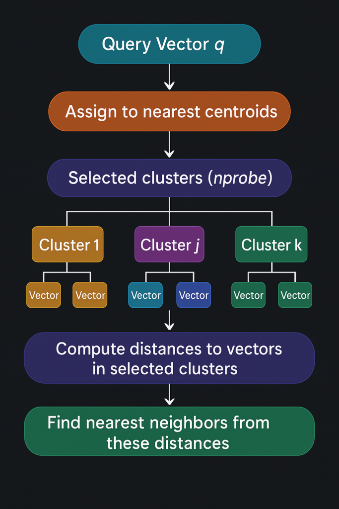
An Inverted File Index (IVF) is a popular technique to speed up vector similarity search by reducing the search scope through clustering. Instead of comparing the query vector with every vector in the dataset (as in a Flat Index), IVF organizes vectors into clusters (also called “buckets” or “centroids”), significantly reducing the number of comparisons during search.
How It Works:
Indexing Phase (Training):
Clustering the Dataset:
- The entire dataset is partitioned into
nlistclusters using a clustering algorithm like k-means. - Each cluster is represented by a centroid (the mean vector of the cluster).
- Each vector in the dataset is assigned to the nearest centroid, forming clusters.
Storing Vectors in Clusters:
- The vectors are stored in an inverted index, where each entry corresponds to a cluster and contains the list of vectors assigned to that cluster.
Search Phase:
Assigning Query to Clusters:
- When a query vector arrives, it is assigned to its nearest centroid(s).
- Instead of searching the entire dataset, the search is conducted within the vectors assigned to the closest clusters.
Advantages of IVF:
- Reduced Search Time: By limiting the search to a subset of clusters, IVF significantly speeds up queries compared to a Flat Index.
- Scalability: More suitable for large datasets than exhaustive search methods.
- Flexibility: By adjusting
nlistandnprobe, you can balance between speed and accuracy.
Disadvantages of IVF:
- Reduced Accuracy: Since the search is limited to selected clusters, some nearest neighbors may be missed.
- Requires Training: The clustering step requires training data and computational resources.
- Parameter Sensitivity: Performance depends on the careful tuning of
nlistandnprobe.
Parameters Affecting Search:
nprobe: Number of clusters to probe during search.- By searching multiple clusters, you can balance between search speed and accuracy.
Parameter Tuning:
Choosing nlist:
- A common heuristic is to set
nlistproportional to the square root of the number of vectors (nlist ≈ √num_vectors). - For
num_vectors = 1,000,000,nlistcould be around1,000.
Choosing nprobe:
- Start with a small
nprobe(e.g., 1% ofnlist) and increase until acceptable recall is achieved. - There’s a trade-off between search speed and accuracy.
Memory Usage Estimation:
The memory requirement for an IVF index can be estimated using the formula:
Memory ≈ 1.1 * (((4 * d) * num_vectors) + (4 * nlist * d)) bytes
Where:
d: Vector dimensionnum_vectors: Number of vectorsnlist: Number of clusters
Example Calculation:
Let’s assume:
d = 128(vector dimension)num_vectors = 1,000,000(number of vectors)nlist = 10,000(number of clusters)
Plugging in the values:
Memory ≈ 1.1 * (((4 * 128) * 1,000,000) + (4 * 10,000 * 128)) bytes
Memory ≈ 1.1 * ((512 * 1,000,000) + (512 * 10,000)) bytes
Memory ≈ 1.1 * (512,000,000 + 5,120,000) bytes
Memory ≈ 1.1 * 517,120,000 bytes
Memory ≈ 568,832,000 bytes (approximately 569 MB)
Ideal Use Case:
- Large datasets where some approximation is acceptable to gain speed.
Product Quantization
Overview:
Product Quantization is a powerful technique to compress high-dimensional vectors into a compact representation, significantly reducing memory usage and accelerating distance computations during search. Unlike dimensionality reduction methods that reduce the number of dimensions (d), PQ maintains the original dimensionality but compresses the data within each dimension by quantizing the vector space.
How It Works:
Indexing Phase:
Vector Splitting:
- Each original vector of dimension
dis divided intomequal-sized sub-vectors. - Each sub-vector has a dimension of
d' = d / m.
Sub-vector Quantization:
- For each of the
msub-vector groups, a separate codebook (set of centroids) is created. - These centroids are obtained by clustering the sub-vectors using algorithms like k-means.
- The number of centroids per sub-vector is
k = 2^b, wherebis the number of bits allocated per sub-vector.
Encoding Vectors:
- Each sub-vector is replaced with the index of the nearest centroid in its corresponding codebook.
- The original vector is thus represented by
mcentroid indices.
Compressed Representation:
- The compressed vector now requires only
m * bbits. - This reduces memory requirements and speeds up distance computations.
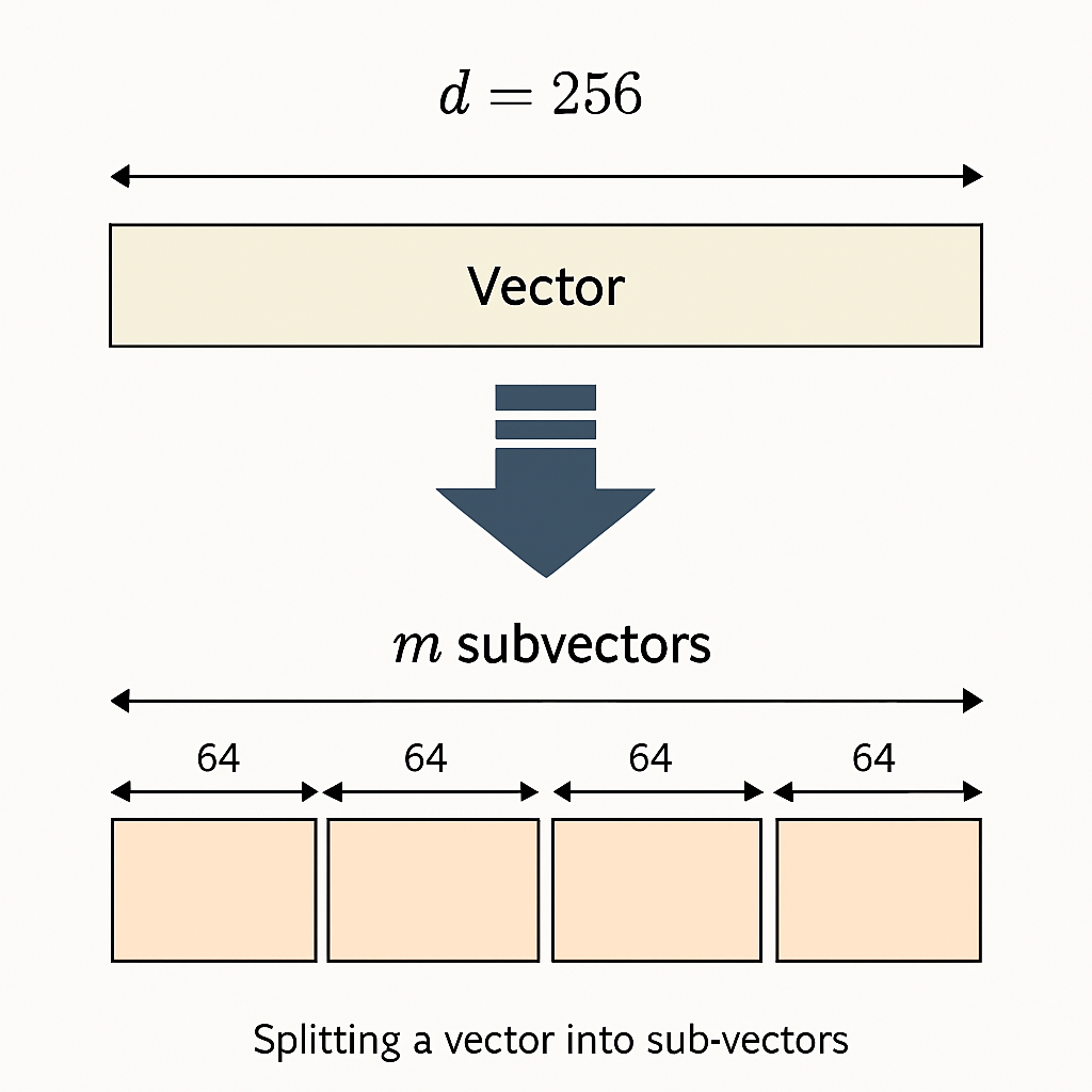
Each vector is split into sub-vectors.
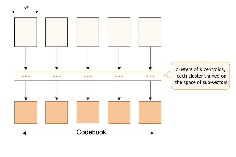
Which are then quantized to centroids (C1, C2, etc.).
Search Phase:
Distance Computation during Search:
During a search, to compute the approximate distance between a query vector Q and a database vector V, the algorithm:
- Splits
Qintomsub-vectors:Q = [Q1, Q2, ..., Qm] - For each sub-vector
Qi, computes the distance to all centroids in the corresponding codebook. - Precomputes a distance table of size
m x k. - Computes the total distance as the sum of distances between
QiandC_Vi, whereC_Viis the centroid representing thei-th sub-vector ofV.
Mathematically:
Approximate Distance(Q, V) = Σ_{i=1}^m distance(Qi, C_Vi)
Advantages of PQ:
- Memory Efficiency: By representing vectors with compact codes, PQ drastically reduces memory consumption.
- Fast Distance Computation: Leveraging precomputed distances accelerates the search process.
- Scalability: Suitable for very large datasets where storing full-precision vectors is impractical.
Disadvantages of PQ:
- Reduced Accuracy: Compression introduces quantization errors, potentially reducing search recall.
- Complexity in Implementation: Requires careful tuning of parameters (
m,b) and proper training of codebooks. - Training Overhead: Building codebooks involves clustering, which can be computationally intensive.
Parameter Tuning:
Choosing m:
- Must divide
devenly. - Larger
mincreases the granularity of quantization, improving accuracy but increasing the size of codebooks.
Choosing b:
- More bits per sub-vector (
b) improve accuracy but increase memory usage for the compressed codes. - Common values are 4, 8 bits.
Number of Centroids k:
- Determined by
k = 2^b. - A larger
kmeans more centroids, leading to finer quantization.
Memory Usage Estimation:
The memory requirement for storing the compressed vectors:
Memory ≈ num_vectors * m * b / 8 bytes
Example Calculation:
Given:
num_vectors = 1,000,000m = 16b = 8bits
Calculating:
Memory ≈ 1,000,000 * 16 * 8 / 8 bytes
Memory ≈ 1,000,000 * 16 bytes
Memory ≈ 16,000,000 bytes (approximately 16 MB)
This is a substantial reduction compared to storing the original 128-dimensional vectors in 32-bit floats:
Memory (Original) = num_vectors * d * 4 bytes
Memory (Original) = 1,000,000 * 128 * 4 bytes
Memory (Original) = 512,000,000 bytes (approximately 512 MB)
Ideal Use Case:
- Very large datasets where memory is a significant concern, and some loss in accuracy is acceptable.
Hierarchical Navigable Small World Graphs
Overview
Hierarchical Navigable Small World Graphs (HNSW) is an efficient graph-based indexing method that offers high accuracy and speed for large-scale approximate nearest neighbor searches. It constructs a multi-layered navigable small world graph that allows for efficient traversal and retrieval of nearest neighbors.
How It Works
Graph Construction:
- Layers: HNSW builds a hierarchy of layers where each higher layer is a sparser graph containing a subset of the nodes from the layer below.
- Connections: Each node (data point) is connected to a limited number of other nodes (neighbors) within the same layer based on proximity.
- Insertion: When adding a new node, it’s inserted into several layers up to a maximum layer determined probabilistically.
- Navigability: The connections are established in a way that the graph exhibits small-world properties, allowing for efficient navigation.
Vectors are organized in multiple layers. Each higher layer is a sparser graph that helps navigate to the bottom layer efficiently.
Search Process:
- Starting Point: The search begins at the top layer with an entry point node.
- Greedy Search: At each layer, the algorithm moves to the neighbor node that is closest to the query vector, using a greedy approach.
- Layer Transition: Once the closest node at the current layer is found, the search proceeds to the next lower layer, using the current closest node as the new starting point.
- Final Search: At the lowest layer, the algorithm explores the local neighborhood to find the approximate nearest neighbors.
Advantages of HNSW:
- High Accuracy: Provides search results comparable to exact methods.
- Fast Search Speed: Achieves logarithmic search time complexity.
- No Training Required: Does not require a separate training phase like clustering.
Disadvantages of HNSW:
- High Memory Usage: The graph’s additional connections consume more memory.
- Complexity: More complex to understand and implement compared to simpler indexing methods.
Parameters and Their Impact:
M (Max Connections per Node):
- Controls the number of bi-directional links per node in the graph.
- Higher
Mimproves the accuracy of the search but increases memory usage and indexing time.
efConstruction:
- Controls the number of neighbors considered during the construction of the graph.
- Higher values lead to better graph quality (higher accuracy) but increase indexing time.
efSearch:
- Controls the size of the dynamic candidate list during searching.
- Higher values improve recall (accuracy) at the expense of longer search times.
Parameter Tuning:
Choosing M:
- Typical values range from 5 to 48.
- Higher
Mincreases accuracy but also memory usage and indexing time.
Setting efConstruction:
- Commonly set between
100and200. - Higher values improve the graph quality.
Setting efSearch:
- Should be set higher than
M. - Increasing
efSearchimproves recall at the cost of search speed.
Memory Usage Estimation:
The memory requirement for an HNSW index can be estimated using:
Memory ≈ 1.1 * (4 * d + 8 * M) * num_vectors byte
Where:
d: Vector dimensionM: Maximum number of connections per nodenum_vectors: Number of vectors
Example Calculation:
Assuming:
d = 128M = 16num_vectors = 1,000,000
Calculating:Memory ≈ 1.1 * (4 * 128 + 8 * 16) * 1,000,000 bytes
Memory ≈ 1.1 * (512 + 128) * 1,000,000 bytes
Memory ≈ 1.1 * 640 * 1,000,000 bytes
Memory ≈ 704,000,000 bytes (approximately 704 MB)
Ideal Use Case:
- Large datasets needing fast and accurate searches, and where memory usage is less of a concern.
Composite Index
Vector indexes are composable. Several indexing techniques can be combined to achieve desired output with acceptable trade-offs in cost, speed or accuracy.
IndexIVFFlat
Partitions the index into multiple buckets. The given (query) vector is first matched to a bucket, then IndexFlatL2 search is performed in this bucket. So the scope of the search is significantly reduced, this means the query time improves but the accuracy of the results go down. Since this method clusters the vectors into multiple buckets, it requires an additional training step.
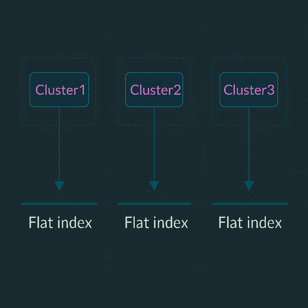
Uses IVF to cluster vectors and Flat Index within each cluster.
IndexIVFPQ
Like IndexIVFFlat, IndexIVFPQ partitions the index into nlist buckets and compresses vectors using PQ. This results in faster query time and less memory consumption compared to IndexFlatL2. However, it comes at a cost of reduced search accuracy. This index also requires training. We can use this formula to calculate the memory requirement for IVF-PQ index:
1.1 * ((((m/8) * m + overhead_per_vector) * num_vectors) + (4 * nlist * d) + (2 m * 4 * d)
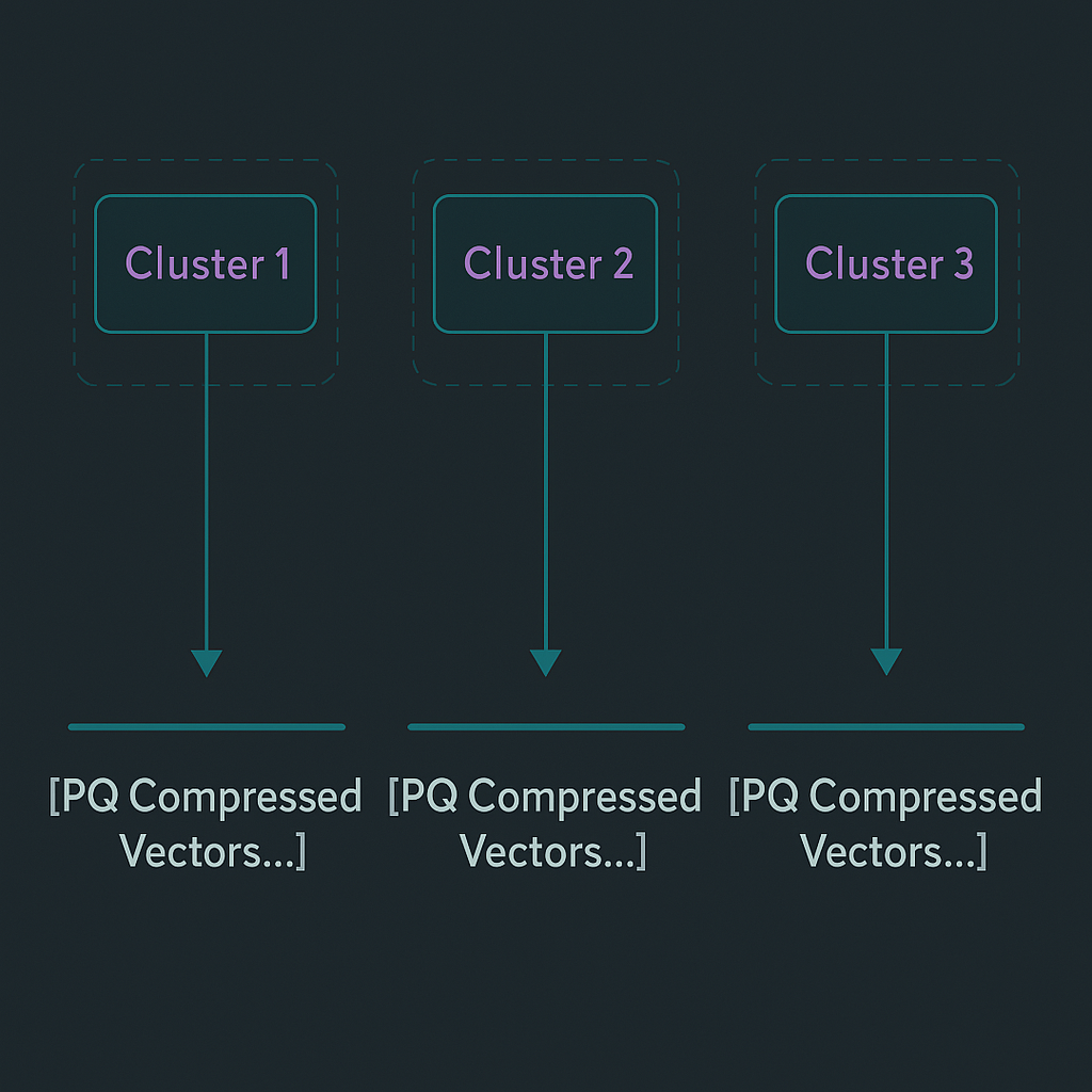
Uses IVF for clustering and PQ for compression within clusters.
IndexHNSWFlat
A HNSW graph stored in a flat list (just like the Flat index) with no other vector compression or quantization.
HNSW Graph Layers
     |
[Flat Index]
HNSW graph built over a Flat Index without additional compression.
Choosing an index
Choosing an index is mainly a trade between these four factors:
- Query Speed: How fast you need the search results.
- Accuracy (Recall): The quality of the search results.
- Memory Usage: The amount of RAM you’re willing or able to use.
- Indexing Time: How long it takes to build the index.
Decision-Making Guide
If Exact Results (Recall = 1.0):
- Use: Flat Index
- When: Small datasets where accuracy is paramount.
If RAM Is Not a Concern OR dataset is small
- Use: HNSW
- Tune:
mandef_searchfor speed-accuracy trade-off.
If RAM Is Not a Concern OR dataset is large
- Use: IVFPQ
- Tune: Set
nlist=1024; adjustm,k_factorfor PQ, andnprobefor IVF.
If RAM Is a Concern:
- Use: IVFFlat
- Tune:
nprobefor speed-accuracy trade-off.
If Memory Is Very Limited:
- Use: PQ Techniques or Dimensionality Reduction (e.g., OPQ)
Clustering Considerations
For each of these techniques, adding clustering can improve search time at the cost of increased indexing time.
For Datasets < 1 Million Vectors:
- Use: IVF
- Set
K: Between4 * sqrt(N)and16 * sqrt(N), whereNis the number of vectors andKis number of IVF clusters. - Training Vectors Needed: Between 30*K and 256*K vectors for training (the more the better).
For Datasets Between 1M and 10M Vectors:
- Use: IVF in combination with HNSW. HNSW to do the cluster assignment.
- Set
M: 32, whereMis maximum number of connections per node in HNSW graph. - Set
K: 65,536, whereKis number of IVF clusters. - Training Vectors Needed: Between
30 * 65,536and256 * 65,536vectors for training.
For Datasets Between 10M and 100M Vectors:
- Use: IVF in combination with HNSW. HNSW to do the cluster assignment.
- Set
M: 32, whereMis maximum number of connections per node in HNSW graph. - Set
K: 2¹⁸ = 262,144, whereKis number of IVF clusters. - Training Vectors Needed: Between
30 * 262,144and256 * 262,144vectors for training.
For Datasets Between 100M and 1B Vectors:
- Use: IVF in combination with HNSW. HNSW to do the cluster assignment.
- Set
M: 32, whereMis maximum number of connections per node in HNSW graph. - Set
K: 2²⁰ = 1,048,576, whereKis number of IVF clusters. - Training Vectors Needed: Between
30 * 1,048,576and256 * 1,048,576vectors for training.
Frequently Asked Questions (FAQ)
Q: Do I always need to train my index?
A: Not necessarily. Indexes like HNSW and Flat Index do not require training. However, indexes like IVF and PQ-based indexes require a training step to create clusters or quantization centroids.
Q: How do I decide between HNSW and IVF-PQ?
A: If memory is not a major concern and you need high accuracy and speed, HNSW is a good choice. If you’re dealing with very large datasets and need to conserve memory, IVF-PQ might be more appropriate.
Q: What is the impact of vector dimensionality on index performance?
A: Higher dimensionality increases both memory usage and computational complexity. Techniques like PQ and dimensionality reduction can help manage this.
Conclusion
Choosing the right vector index is a critical decision that can significantly impact your application’s performance. By understanding the strengths and limitations of each indexing technique, you can make an informed choice that balances speed, accuracy, memory usage, and indexing time.
Remember:
- Assess Your Needs: Understand your dataset size, dimensionality, and application requirements.
- Balance Trade-offs: Decide what is more critical—speed, accuracy, or memory.
- Experiment and Tune: Use the parameters to fine-tune the index for your specific use case.
Feel free to share your thoughts or ask questions below—let’s continue the conversation!
Leave a Reply