Chirag Agrawal
Senior software engineer / ML systems / developer tooling
I have been building large scale conversational AI systems for the past decade. Here I share some notes and show off cool stuff.
Published pieces
09
Open source projects
04
Podcast appearances
03
Publication platforms
06
Latest writing
Published on freeCodeCamp
How to Persist State in Time-Series Models with Docker and Redis
Have you ever built a brilliant time-series model, one that could forecast sales or predict stock prices, only to watch it fail in the real world? Well, this is a common frustration. Your model works perfectly on your machine, but the moment you deploy it in a Docker container, it seems to develop amnesia. It forgets everything it knew yesterday, making its predictions for tomorrow useless.
Open publicationRecent writing
Shipping notes from the workbench.
Slimming Down Docker Images: Base Image Choices and The Power of Multi-Stage Builds
Multi-stage Docker builds separate build-time dependencies from runtime requirements, dramatically reducing production image sizes.
Expert Techniques to Trim Your Docker Images and Speed Up Build Times
Use -slim base images, multi-stage builds, smart layer caching, and chained RUN commands to build lean, fast, and production-ready Docker images.
Make Docker Builds Faster with Layer Caching
Dockerfile is an immutable ledger. Look at it this way and optimizing containers becomes intuitive and obvious.
Personal Projects
Tools built around containers, inference, and practical AI.
docker-redis-time-series
A simple demonstration of time series prediction using ML model and redis db hosted in Docker container.
docker-transformers-inference
A containerized solution for hosting transformer models using Flask, Gunicorn, and Docker with AWS SageMaker deployment support. Build once, run anywhere!
ai-docker-image-optimization
A evolving codebase that demonstrates various techniques to optimize docker image for size and performance.
Podcast appearances
Conversations on architecture, agentic systems, and developer experience.
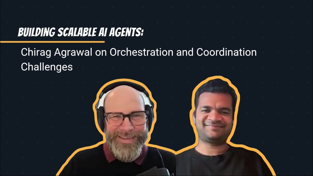
Building Scalable AI Agents: Chirag Agrawal Explains How
I joined the Beginner's Guide to AI podcast to break down how to build scalable AI agents — covering architecture patterns, orchestration strategies, and practical lessons from production deployments.
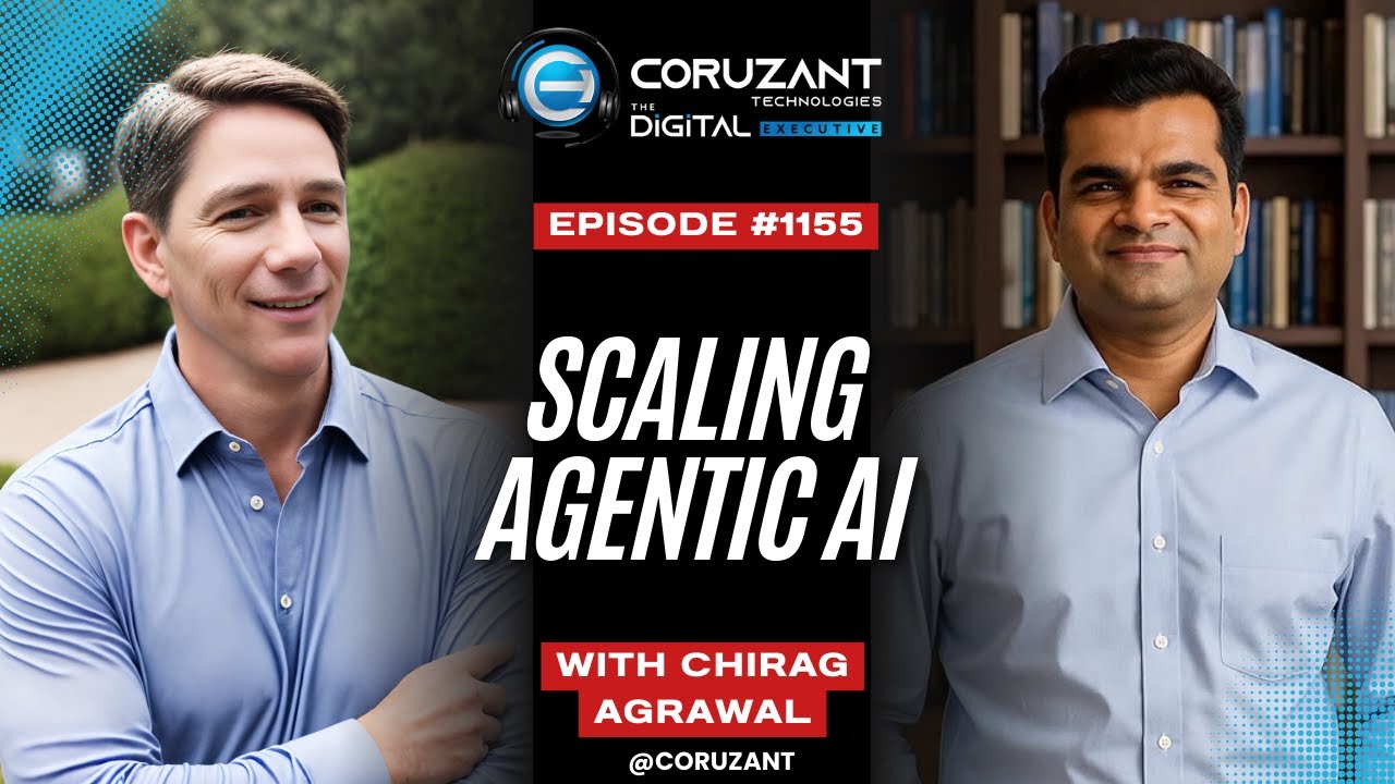
Scaling Agentic AI with Chirag Agrawal
I spoke with The Digital Executive about scaling agentic AI systems — discussing the challenges of building autonomous AI agents that operate reliably at enterprise scale.